Data Modeling

Introduction

With Dojo's Data Modeling tool, users can combine NetCDF datasets together through a simple visual programming interface to create new and insightful derived datasets.

Relatively complex data operations and transformations can be performed on a variety of different kinds of data, no programming skills required.

Selecting NetCDFs

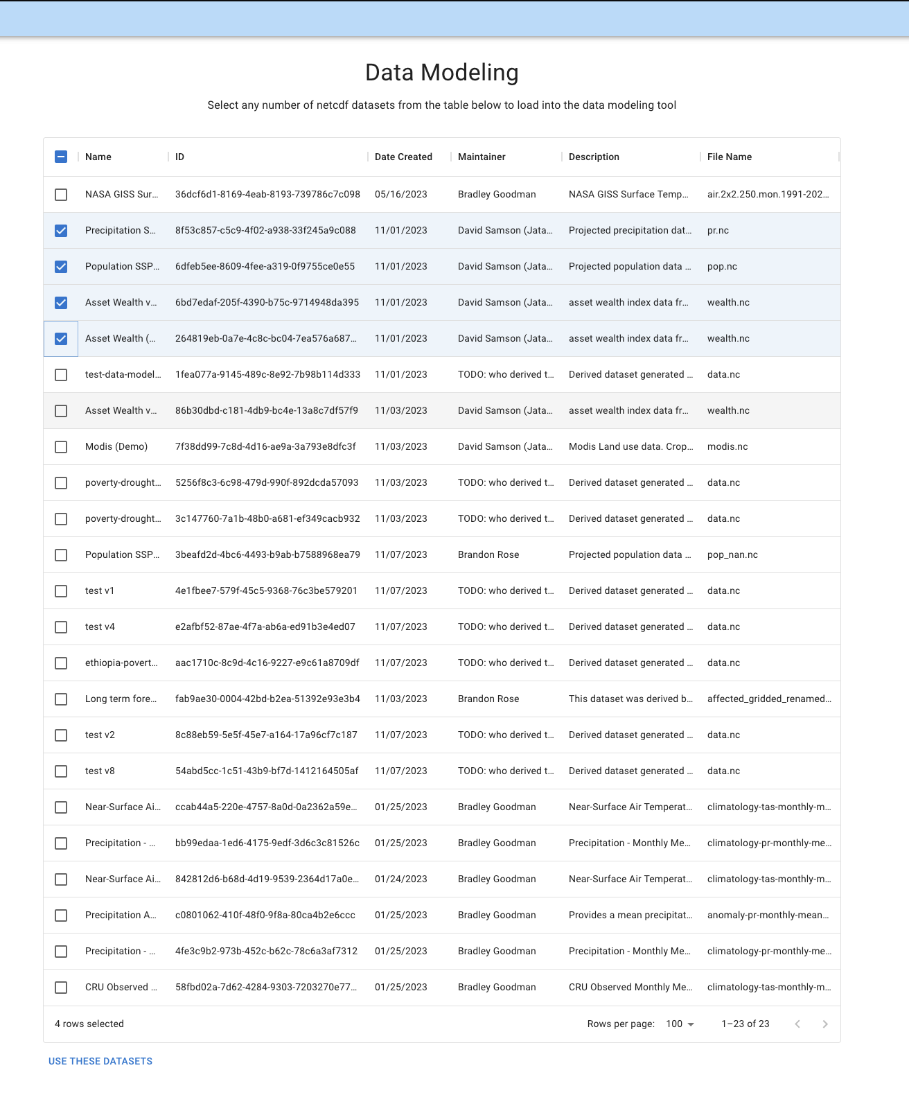
When you initially land on the Data Modeling page, you'll be prompted to selected registered NetCDFs. If you have a NetCDF that you'd like to use that isn't yet registered in Dojo, follow the steps in Data Registration to register it. It will then appear in the list of NetCDF datasets.

You can select as many datasets as you'd like. Once you've selected all your datasets, click USE THESE DATASETS on the bottom of the page to move to the next step.

Building a Graph

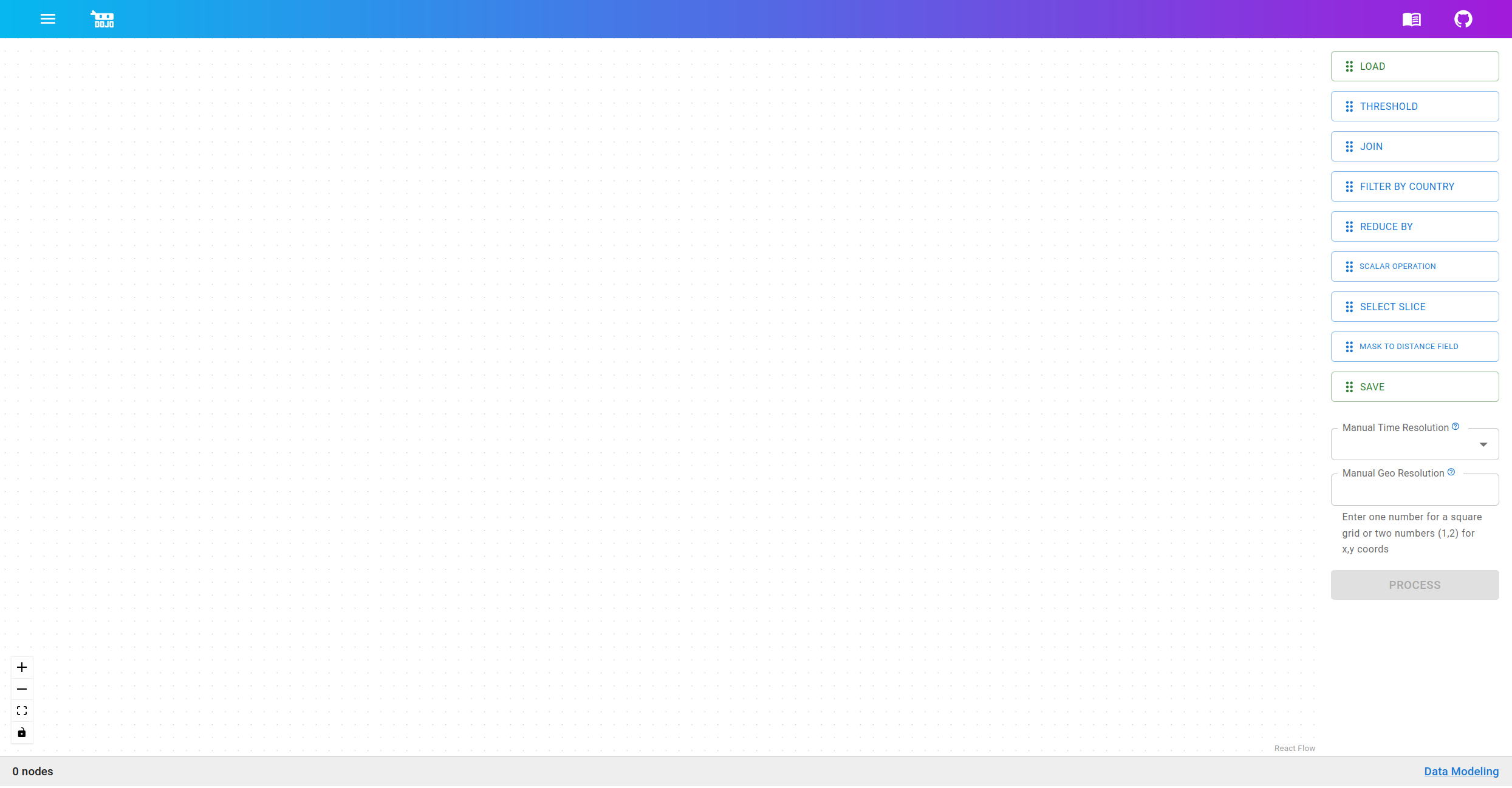
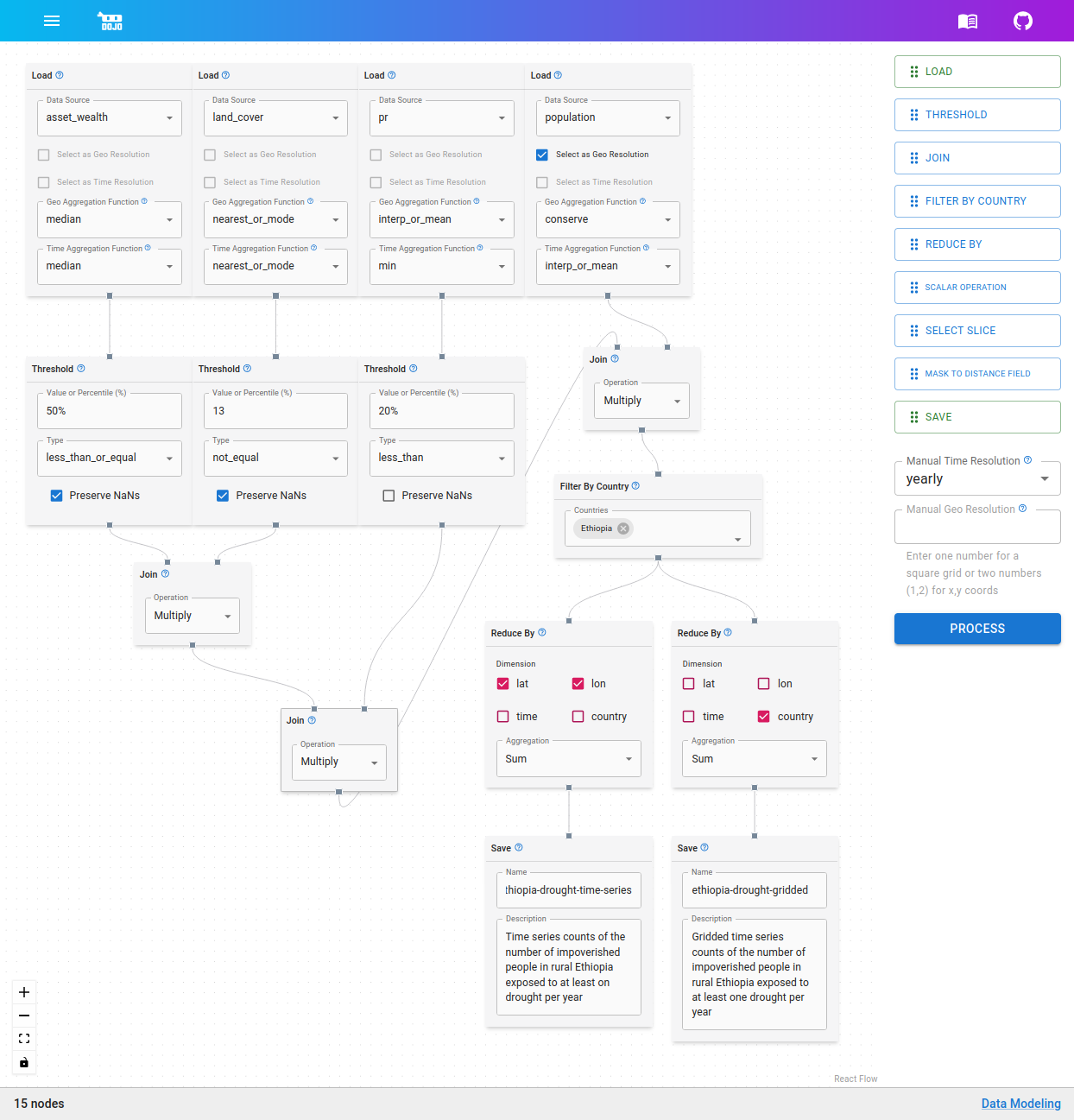
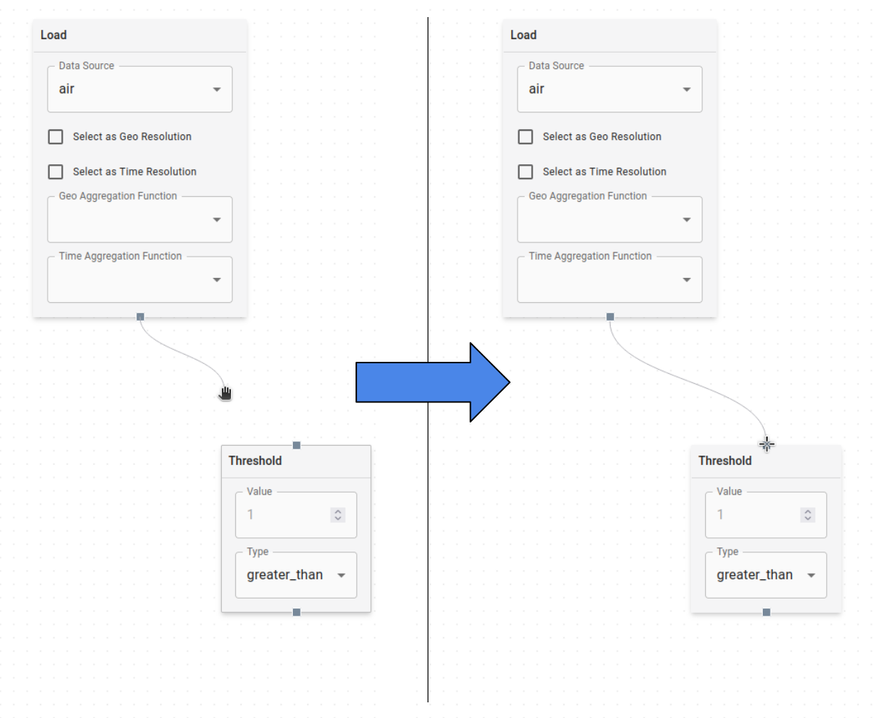
On the second step, you can start building out your data graph. Drag and drop nodes (explained in further detail below) from the node selection panel on the right side of the screen onto the blank canvas area on the left. Once nodes are on the canvas, they will appear with small connection points on the top and/or bottom (inputs and outputs respectively). You can click and drag between these connection points to apply operations to the data.

Adding multiple nodes and creating a network of connections between them defines how input data should be transformed by the data flow graph to create the derived output data.

Nodes:

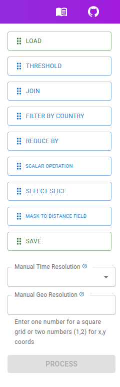
Node List

This is the current list of nodes available for building a data modeling graph.

Load Node

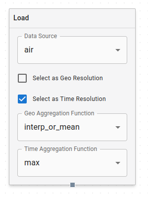
Load Node

The Load Node is how data is brought into the data modeling process. Each Load Node represents one feature from a dataset. You select this feature with the Data Source dropdown at the top of the node. You'll see features listed per dataset in this dropdown.

The following options in the Load Node relate to how data regridding is handled.

The first of these is a global target resolution that applies to all your features. You need to select both a geo and temporal target resolution. You can either manually hardcode these (see Manual Resolution below), or you can check one or both of the boxes on a Load Node to make its resolution be the target resolution. For the entire graph, you can only have one geo and one temporal target resolution, either in the Load Nodes or in the manual selectors in the sidebar.

The second is selecting regridding methods that will be used if the data in the load node needs to be regridded. These are specified with the Geo and Time Aggregation function dropdowns for each Load Node:

• conserve - maintain the total sum of the data before and after (e.g. for regridding population)
• min - take the minimum value from each bucket during regridding
• max - take the maximum value from each bucket during regridding
• mean - take the mean value from each bucket during regridding. Note: Use interp_or_mean instead of mean, since it doesn't handle well when increasing the resolution of the data
• median - take the median value from each bucket during regridding
• mode - take the mode of each bucket during regridding. Note: Use nearest_or_mode instead of mode, since it doesn't handle well when increasing the resolution of the data
• interp_or_mean - if increasing resolution, interpolate the data. If decreasing resolution, take the mean of each bucket
• nearest_or_mode - if increasing resolution, take the nearest data. if decreasing resolution, take the mode of each bucket

Threshold Node

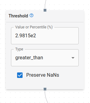
Threshold Node

Threshold Nodes are used to select specific portions of data where some condition is true.

Take the example of a temperature dataset where you want to filter for values above a threshold temperature. A Threshold Node that takes temperature data as input and is set to greater_than with the value of your threshold creates a boolean mask that is true wherever the condition was met. This can then be used to filter the original data with a Join Node.

Threshold values can be an integer or floating point number, and may optionally end with a percent (%) symbol. Some examples:

• 42
• -5345
• 10%
• 0.0003
• 1.34e12
• 99.9%
• 1.63e-6%

The percent symbol indicates a percentile threshold. Percentile thresholds must be between 0 and 100, and will automatically calculate the correct data value to apply the threshold for the specified percentile. Otherwise, the threshold value is applied directly to the data.

The type of comparison operation (=, ≠, >, ≥, <, ≤) is specified with the dropdown menu.

The checkbox for Preserve NaNs indicates how the threshold should be applied to NaN values in the data. If checked, any NaN values in the original data will be carried forward unmodified by the threshold. If unchecked, NaN values will be converted to False in the threshold operation.

Join Node

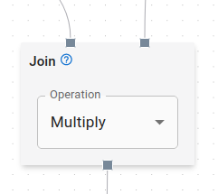
Join Node

Join Nodes are used to combine multiple nodes in the graph into a single dataset. Join Nodes take as input two parent nodes and output the values of those input nodes combined together. The particular operation used to combine the datasets is specified via the dropdown menu. The options are Add, Subtract, Multiply, Divide, and Power. The output of a Join Node is calculated as follows:

output = left_parent <operation> right_parent

note

For the non-commutative operations Subtract, Divide, and Power, it is important to ensure the order of the parent nodes is correct.

The most common use case for Join Nodes is to filter data to where some condition is true. A dataset mask can be created with a Threshold Node, and then that mask can be "joined" with the data that you want to apply the mask to using the multiply aggregation.

Other join operations are used to combine datasets in other ways. For example say you have two datasets, one with population by country, and with with land area by country. You could use a Join Node with the Divide operation to get a new dataset that is population density by country. The particular operation you should use will depend on the data you're working with and the analysis you're trying to perform.

Filter By Country Node

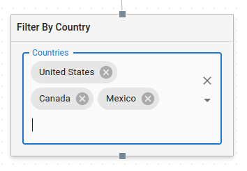
Filter By Country Node

With this node, you can filter the data coming out of your selected features by the countries you select in the dropdown. You can select multiple countries. The output dataset will be a copy of the input dataset, but with an extra admin0 (i.e. country) dimension. Every country specified in the Filter By Country Node will be split into its own separate layer along the country dimension of the output. All other values not within the bounds of any of the specified countries will be set to 0.

note

Data input into this node must have lat, and lon dimensions, as these are used to determine which data points are within the bounds of the specified countries.

note

This node does not remove any existing dimensions, so the output will have lat, lon, and admin0 dimensions, and optionally time if the input data had a time dimension.

Reduce By Node

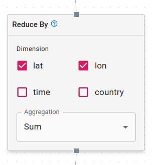
Reduce By Node

This node can be used to aggregate a dataset across one or more dimensions. The input dataset will be reduced along the dimensions specified by the checkboxes, according to the selected aggregation method. Aggregation methods include Sum, Mean, Median, Min, Max, Standard Deviation, and Mode.

For example, say you have monthly population data gridded to 0.1x0.1 lat/lon, and you would like to produce a single population curve over time. Using the Reduce By Node, selecting lat and lon as the dimensions, and selecting Sum as the aggregation will sum up all of the values for each time slice in the input dataset, and produce a new dataset that is just a single aggregated curve over time.

tip

At present, Reduce By Nodes are hardcoded with the options lat, lon, time, and country, regardless of what dimensions your data has. Take care to only select dimensions that actually exist on your dataset.

Scalar Operation

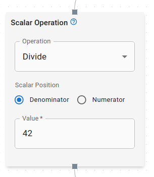
Scalar Operation Node

Scalar operations provide a simple node for applying scalar operations to your data. The scalar value can be set in the input field, and the operation can be selected from the dropdown menu. The available operations are Add, Subtract, Multiply, Divide, and Power. For the simple operators (Add, Subtract, Multiply), the result is calculated as follows:

output = input <operation> scalar

For Divide and Power, you have a radio selector for specifying the position of the scalar in the operation. For Divide, you may select either Numerator or Denominator, giving the following results:

// Divide with scalar position set to 'numerator'
output = scalar / input

// Divide with scalar position set to 'denominator'
output = input / scalar

For Power, you may select either Base or Exponent, giving the following results:

// Power with scalar position set to 'base'
output = scalar ^ input

// Power with scalar position set to 'exponent'
output = input ^ scalar

Select Slice

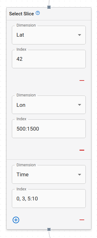
Select Slice Node

Select slice is used to select a slice of data along one or more specified dimensions. The dimension dropdown is used to specify what dimension the slice should be selected from. The index field is used to specify the slice. A slice can be either:

• a single integer
• a range of integers separated by a colon :, e.g. 0:10
• a comma separated list of integers or ranges, e.g. 0, 2, 4:6, 8:10

For example, if you have a dataset with a time dimension, and you want to select only the first 10 time slices, you would use a Select Slice Node with time selected as the dimension, and 0:10 as the index.

Lastly, you can use the +/- buttons to add additional or remove existing slices to the node.

note

if the index is a single integer, then that dimension will be removed from the output dataset. Otherwise, for ranges and more complicated slices, the dimension will be retained in the output dataset.

Mask to Distance Field

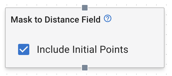
Mask to Distance Field Node

The Mask to Distance Field Node is used to convert a binary mask into a distance field. The input mask is a boolean mask where True values represent the mask, and False values represent the background. The output distance field is a floating point field where each value represents the distance from the nearest True value in the mask. Additionally, any NaN values in the initial data will be carried forward as NaN in the output. The distance field is calculated using the Haversine distance formula over the surface of the Earth.

note

Distances values in the result are in kilometers

If include initial points is checked, then all the initial points in the mask will have a distance of 0. If unchecked, then all initial points will have a distance of NaN.

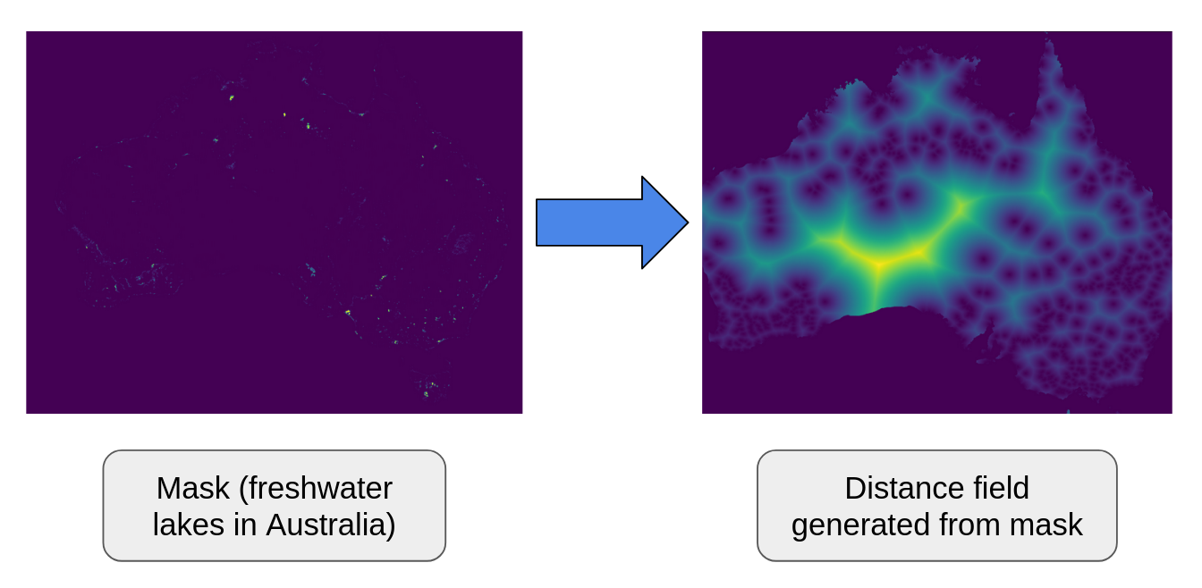
Mask to Distance Field Example

In this example, the left image is a mask over Australia where True values represent locations of freshwater (e.g. lakes, rivers), and False values represent the background. Then the right image is the distance field calculated from the mask. Distances near the initial points are dark, and distances further away are brighter

note

Input to mask to distance field is expected to be a mask with lat and lon dimensions. Masks may either be boolean, or floating point limited to values 0, 1, or NaN. Either your input data must be in mask form, or you must use a Threshold Node to create a mask before using this node.

tip

Mask to distance field will handle additional dimensions (i.e. time, country) by treating each slice as independent. However it is not recommended to used data with additional dimensions, as the calculation will be very slow.

Save Node

Save Node

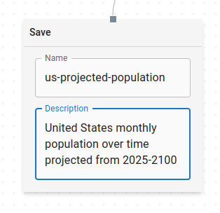
The final step in a graph is adding a Save Node. The Save Node has input text fields for both name and description, which will be used to label the output dataset and save it back into Dojo as a new derived dataset.

Manual Resolution

Manual Resolution

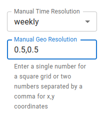
Below the list of nodes on the right side of the screen, you'll find two inputs where you can manually set your Geo and/or Time Resolution. You can use these instead of selecting one of your Load Node features to be Geo/Time Resolution if you want to set the resolution by hand. If you set it here, you won't be able to select any of the same type of resolution elsewhere until you clear it.

tip

Selecting both a Geo and a Temporal Resolution is required before you can process your graph. These can be set manually in the sidebar, in the Load Nodes, or one of each.

Processing

Once you're done setting up your graph, click the PROCESS button to start running the backend process. When it's complete, you'll see a list of the datasets that the process output.

tip

It is important to make sure you have at least one Load Node with a feature selected. Also ensure that all the nodes in your graph are connected before hitting process.